Deep learning and all kind of machine learning techniques have received a lot of attraction recently. However, most of the commonly used tool for data science and machine learning are implemented in python. As the most favorable programming language of statisticians is R, some might hesitate to stay out of their comfort zone.

TensorFlow first releases in 11/2015 as a machine learning framework which is usability and flexibility. In the github folder of TensorFlow, there are several examples on NPL, computer vision … Off course, Tensorflow is natively supported in python. Recently, Rstudio team develops a library for R which is quite interesting.

In this post, I will explain my understanding on how to implement a simple model and have some fun.

Deep learning

In deep learning, we use multi-layer neural networks. In each nodes, there are functions/operations that transform the input (Tensor) to the output (Tensor). As a graphical model, we might have some interest in the gradient of each nodes and Tensorflow will help you with this stage effortlessly.

In the first step, we have to propose a graph model. It might sound complicated but imagine that you have an equation with constants and variables \(y = A x + b\) Then we could describe constants and variables as tensor and operators as nodes. Using Iris data, I assume that x is iris$Petal.Length and y is iris$Petal.Width.

#devtools::install_github("rstudio/tensorflow")
library(tensorflow)
library(ggplot2)

data(iris)
#head(iris)
x_data <- iris$Petal.Length
y_data <- iris$Petal.Width

A <- tf$Variable(c(1),	name="Coefficient")
b <- tf$Variable(c(1),	name="Intercept")
# y <- tf$add(tf$mul(A, x_data), b)
y <- A * x_data + b

So, we have created a Coefficient and Intercept as a variable. As all computation in Tensorflow needs to be called in Session. We obtain the equation using sess$run() as,

sess <- tf$Session()
sess$run(tf$initialize_all_variables()) # To init all the vars
print(sess$run(y))
sess$close()

Well, now we have more or less everything we need for a simple linear regression. Remember that in linear regression, we want to minimized the mean square error.

We need an optimizer method and put the MSE as the objective function. Different from the close form linear regression lm, in the optimization method, we have to loop over the parameter set until we reach the optimal point.

MSE <- tf$reduce_mean((y_data - y)^2)
optimizer <- tf$train$GradientDescentOptimizer(0.03)
train <- optimizer$minimize(MSE)

sess <- tf$Session()
sess$run(tf$initialize_all_variables()) # To init all the vars

for (i in 1:2000) {
    sess$run(train)
}
cat("Coefficient: ", sess$run(A), "\n Intercept: ", sess$run(b), "\n")

## Coefficient:  0.4157551 
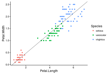
##  Intercept:  -0.363074

We visualize the final result as,

ggplot(iris, aes(Petal.Length, Petal.Width)) + 
    geom_point(aes(color = Species)) +
    geom_abline(slope = sess$run(A), intercept = sess$run(b), alpha = 0.5) + 
    theme_classic()+
    theme(axis.line.x = element_line(color="black", size = 0.5),
          axis.line.y = element_line(color="black", size = 0.5))

sess$close()
# Compare to the lm function
lm(y_data~x_data)

## 
## Call:
## lm(formula = y_data ~ x_data)
## 
## Coefficients:
## (Intercept)       x_data  
##     -0.3631       0.4158

Conclusion

With this ‘not so deep example’, we have experienced that Tensorflow helps to build graphical model and estimate the parameter with a user defined loss function. In this example, we need to tweak the GradientDescentOptimizer(learning_rate). A large value of learning_rate might not guarantee convergence while a smaller one might slow down the convergence of the objective function. More advanced examples could be found at Rstudio website