Lab Review 3
Hoang Nguyen
Feb 17, 2017
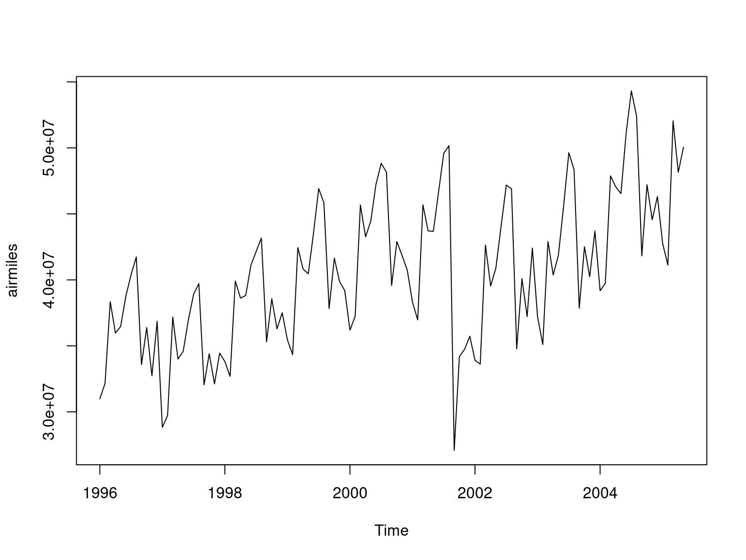
Another example of the Monthly U.S. airline passenger-miles: 01/1996 - 05/2005.
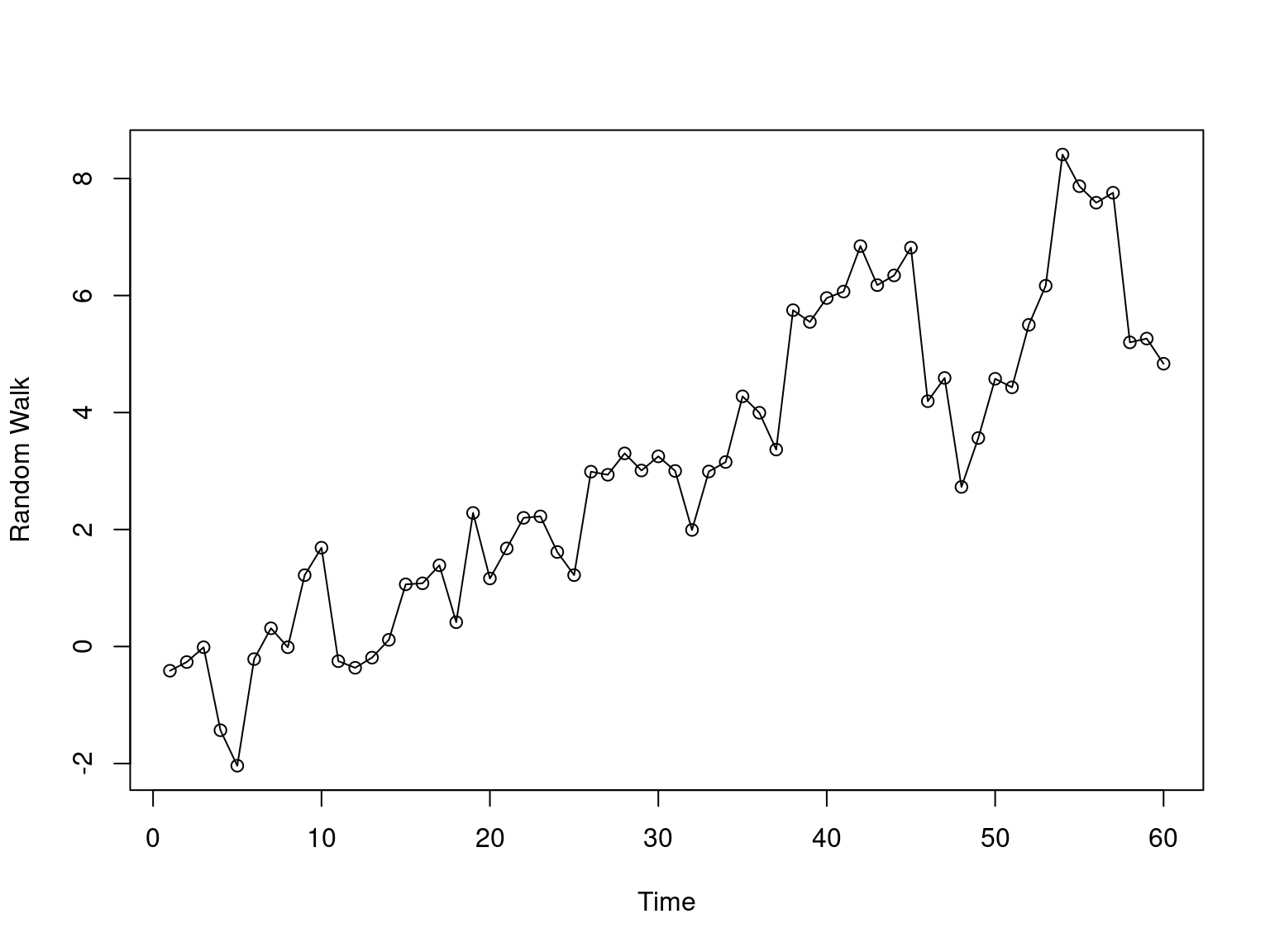
Random walk is stationary?
eps = rnorm(10000)
randomwalk = cumsum(eps)
plot(randomwalk, type = "l")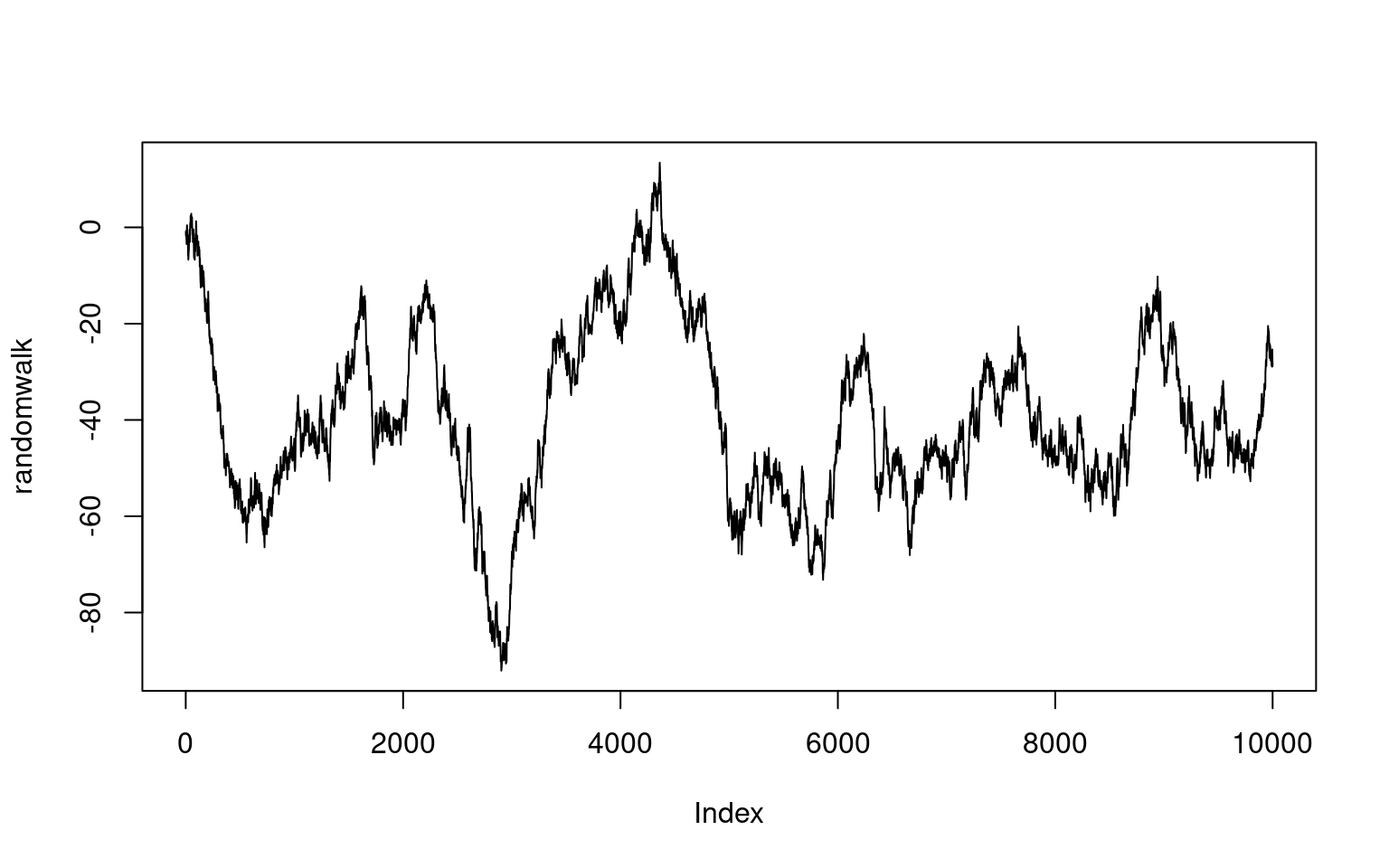
acf(randomwalk)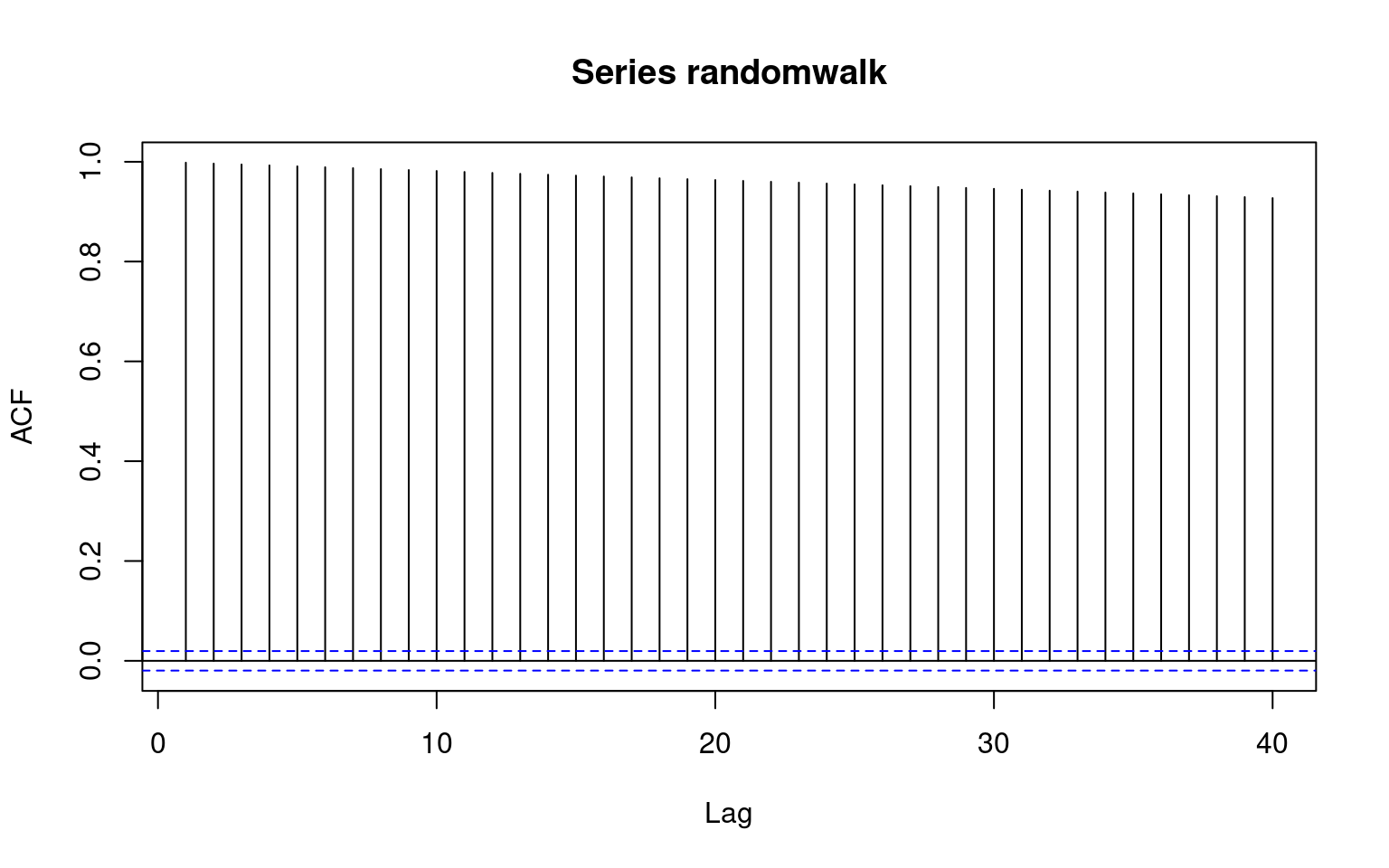
pacf(randomwalk)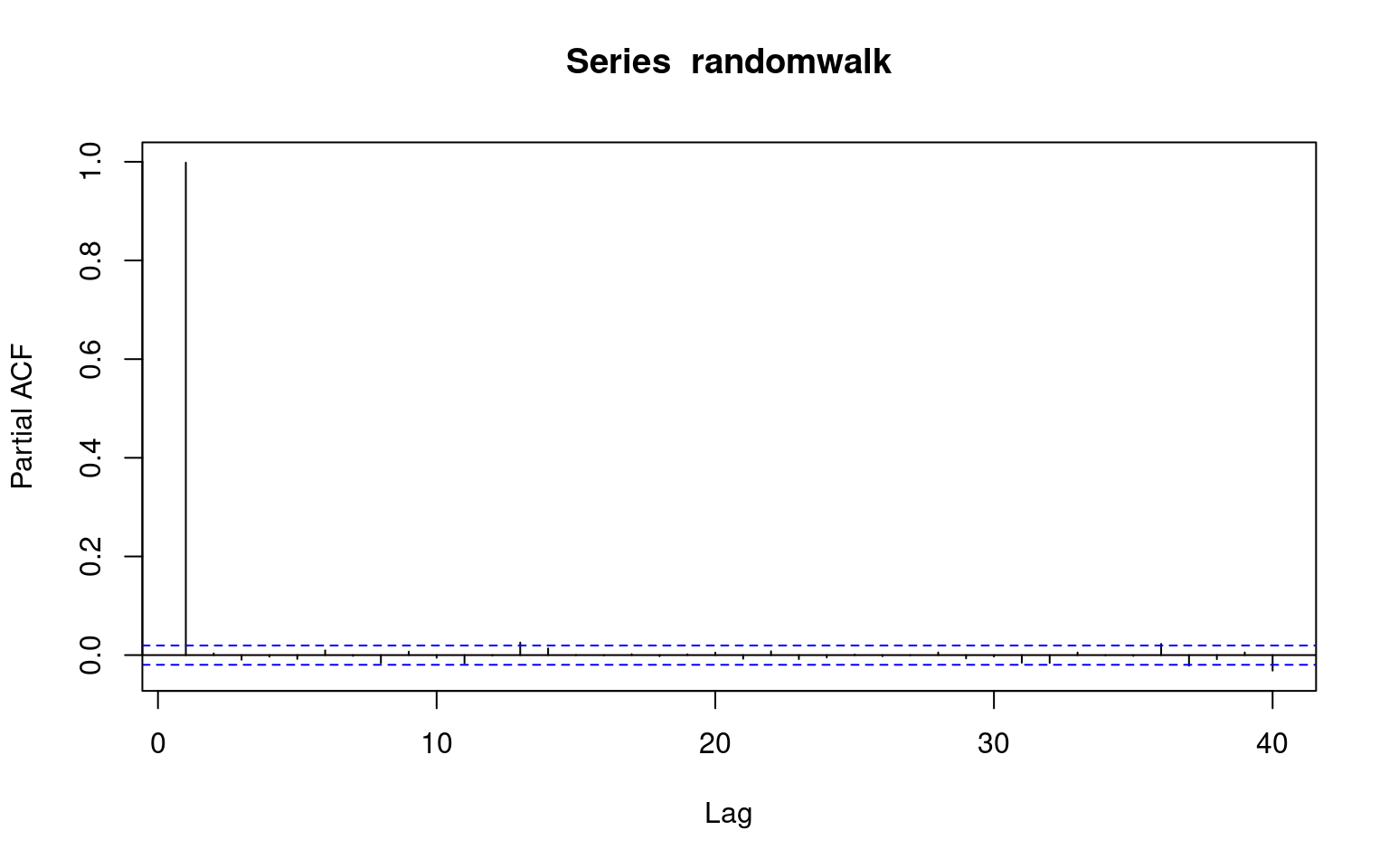
White Noise
plot(eps, type = "l")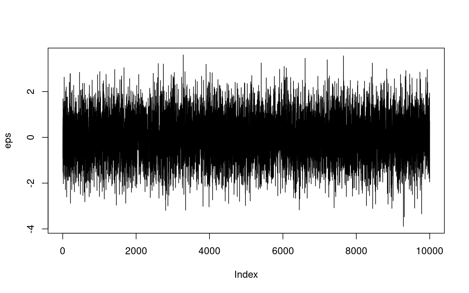
acf(eps)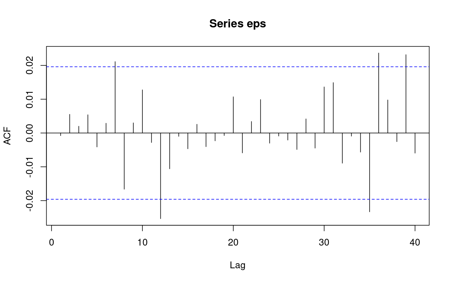
pacf(eps)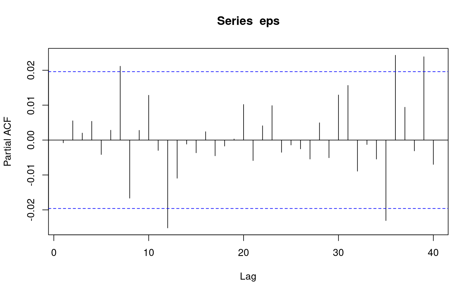
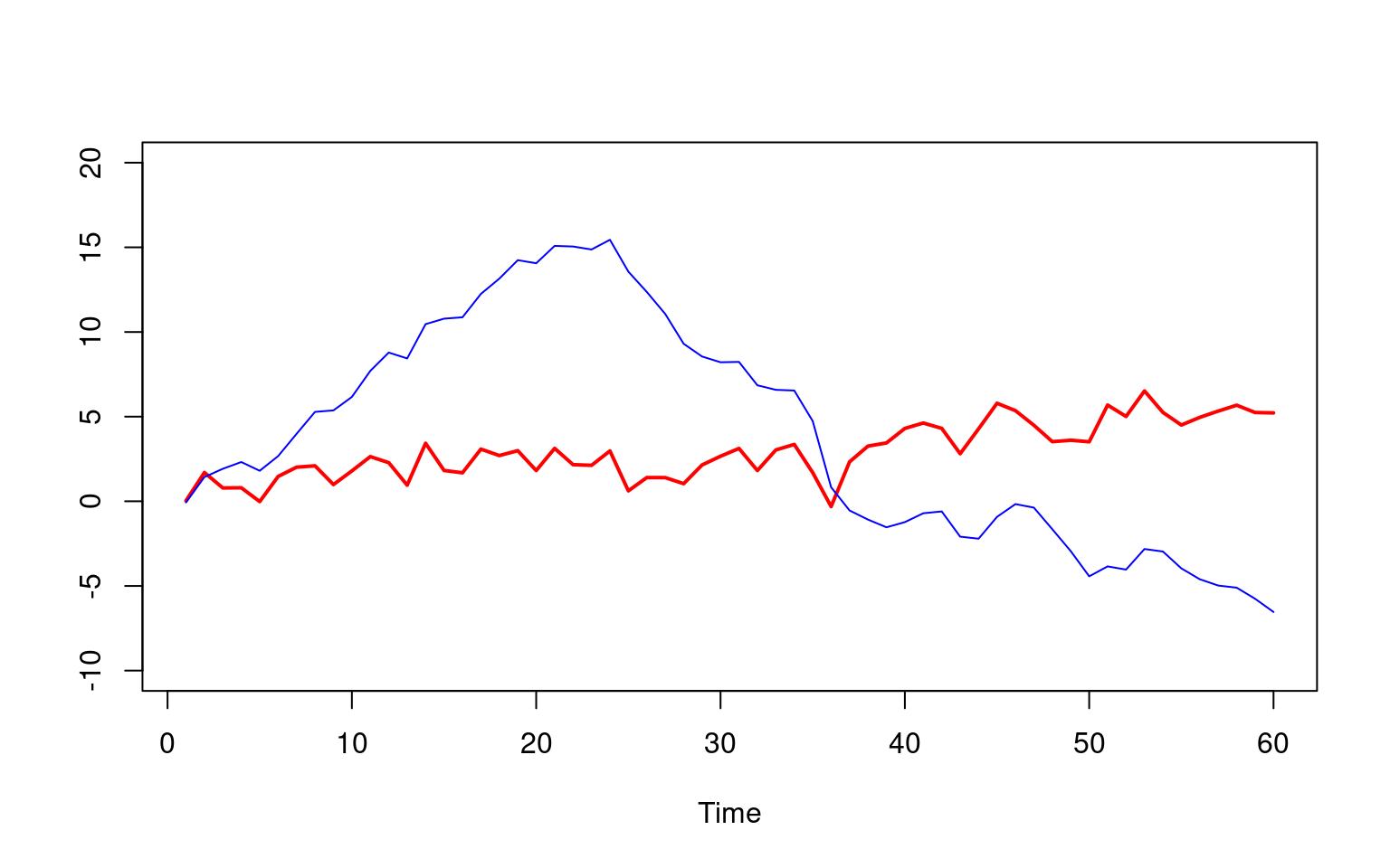
Make your guess?
Trend Stationary or Difference Stationary
acf(trend_stationary)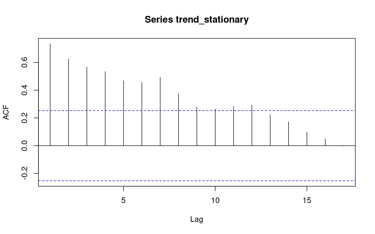
pacf(trend_stationary)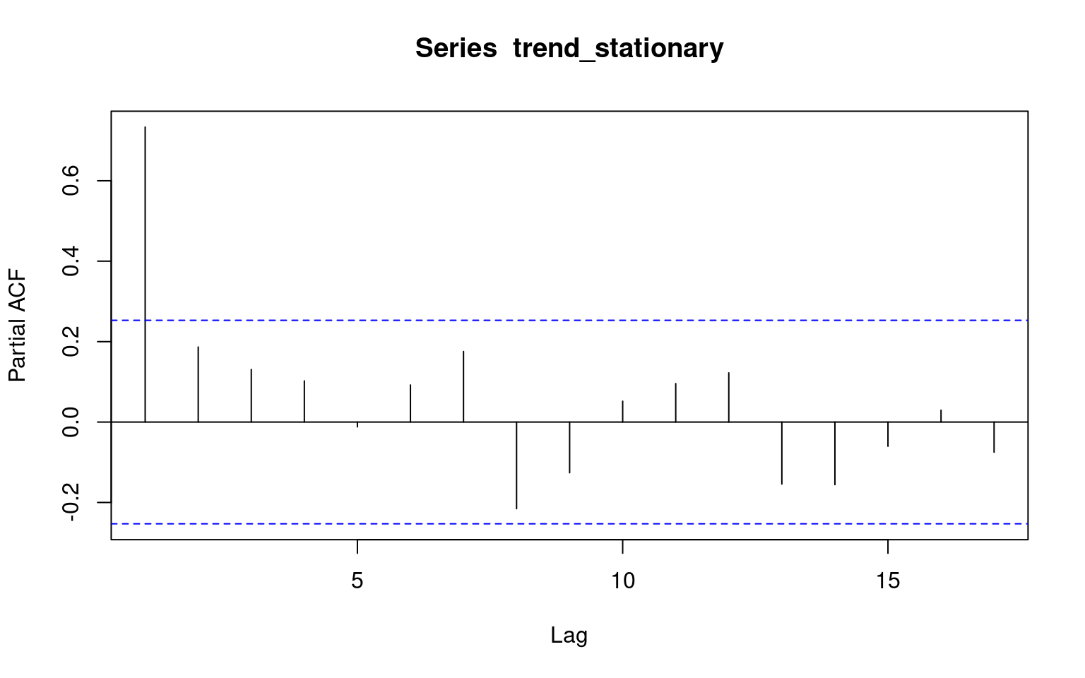
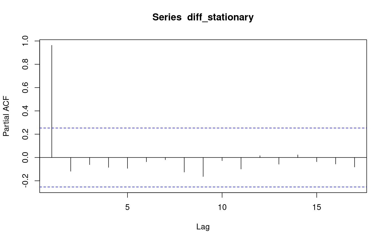
acf(diff_stationary)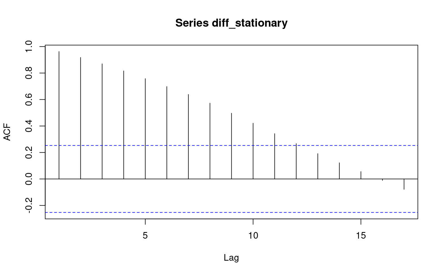
pacf(diff_stationary)